DualPipe Explained: A Comprehensive Guide to DualPipe That Anyone Can Understand—Even Without a Distributed Training Background
Last week, DeepSeek announced an “OpenSourceWeek” on social media, releasing a series of open-source software libraries for five consecutive days. Over the first few days, they introduced FlashMLA (an efficient Hopper GPU MLA decoding kernel), DeepEP (an expert parallel communication library for MoE), and DeepGEMM (a GEMM library with FP8 support). On the fourth day, they open-sourced three major components in one go: DualPipe, EPLB, and profile-data. Among these, DualPipe—due to its core idea of “bidirectional pipeline parallelism”—sparked widespread discussion.
This blog post will focus on the core concept of DualPipe: how to fully overlap forward and backward passes in large-model training, thereby greatly reducing the “bubble time” in pipeline execution. To help you grasp these ideas, we’ll start with a straightforward analogy—“process optimization in a machine workshop”—introducing each concept first through the lens of mechanical processing, and then mapping it back to parallel training in deep learning. By the end of this article, you’ll have a clear picture of how these ideas work. We’ll also delve into DualPipe’s source-code-level details, exploring how it further reduces pipeline bubbles, overlaps forward and backward passes, minimizes communication pressure, and integrates into more complex hybrid parallelism scenarios.
1. Introduction
With today’s buzz around large language models (LLMs) such as GPT-3, PaLM, and LLama, distributed training has become an essential technique for pushing beyond the limits of a single GPU and successfully training ultra-large models. Terms like data parallel, model parallel, and pipeline parallel come up often, yet it can be challenging—especially for beginners—to see how they differ and connect. And when you encounter advanced features like DualPipe in DeepSeek-V3, it might feel even more daunting.
On the other hand, in industrial settings, optimizing a production process often involves countless trials, while in AI, training a large language model similarly requires numerous parameter adjustments. These two activities may seem unrelated, but they share a remarkable resemblance. Let’s walk through a story from Tony’s machine workshop to see how a production line with multiple machine tools can help us understand the four major types of parallelism in large-model training.
1.1 The Single-GPU Era: The Small Handicraft Workshop
In Suzhou Industrial Park, Tony owns a mid-sized mechanical company that focuses on optimizing manufacturing processes such as casting temperature, quenching time, cutting angles, etc. When a new order arrives, Tony first designs a set of initial manufacturing parameters (the “process manual”), proceeds with machining, then inspects the final part and back-propagates the adjustments: if the part has void defects, he tweaks the casting temperature upward, and so on.
Tony’s process is remarkably similar to large-model training: the “process manual” is like the model’s parameters, the parts being machined are akin to training data, each individual process (casting, heat treatment, etc.) corresponds to different layers in a neural network, and the machine tools are analogous to GPUs. Finally, the quality check is akin to computing the loss function, and adjusting parameters based on the inspection is just like backpropagation.
When Tony started his business, he took on relatively simple orders, like machining screws. For such parts, you only need a single multifunctional machine to handle two steps: cutting and polishing. If the part turned out unevenly polished, you’d adjust the polishing step; if the cutting was off, you’d adjust the cutting angle. It was all done on a single machine—like a small handicraft workshop. That was enough for basic parts, but there was no scalability.
This corresponds to single-GPU training. All model layers (all “process steps”) run on the same GPU (the same machine). Both the forward pass (machining) and the backward pass (adjusting parameters) happen on a single device. It’s simple and reliable, but once the tasks become more complex, a single device becomes the bottleneck.
1.2 Model Parallelism: The Art of Splitting the Process Manual
One day, Tony received a much bigger order for optimizing the process of manufacturing an engine crankshaft. He quickly realized that a single machine could not handle all the needed steps. So he split the processes (casting, heat treatment, precision machining) across three specialized machines, each equipped with its own operation instructions. He also had to keep track of how adjusting casting parameters might affect subsequent processes. It introduced a new problem—machine idle time. While the first machine was busy casting, the other machines might be waiting. Plus, moving items from one machine to the next took additional time. If not planned carefully, these machine transitions could cause extra idle periods.
In large language models, this is model parallelism. When a model is too large for a single GPU’s memory, you split it across multiple GPUs (e.g., different layers or different modules for each GPU). In this analogy, the casting is like an input layer, heat treatment is the intermediate layer, and precision machining is the output layer. As you train, each GPU is responsible for a segment of the model and must communicate intermediate outputs to others. This inevitably leads to idle time across GPUs and frequent cross-device data transfer. The problems Tony faces resemble the scheduling and communication challenges among GPUs.
1.3 Data Parallelism: A Plan to Clone the Workshop
To further speed up the process-parameter optimization, Tony—now with more funding—built three identical workshops next door. Each workshop has the same entire pipeline, just working on different batches of turbine discs (data shards). By the end of the day, the four workshop managers come together to compare notes and unify the process standards. An order of 10,000 raw parts that used to take a month now only needs about two weeks. Tony wonders, “Why did quadrupling my workshop capacity only double the speed?” After talking to the managers, he found that each batch of raw materials might encounter unique problems, causing some workshops to finish later. When they’re done, they have to wait for the slowest one before summarizing the day’s results.
This is data parallelism. Each workshop (GPU) holds a full copy of the process manual (model parameters) but processes a different portion of the data (different mini-batches). Once each workshop computes its local gradient (inspecting the part and figuring out parameter adjustments), they must gather and average these gradients (through All-Reduce) to form a unified set of parameters. The bottleneck is that the slowest workshop (straggler GPU) holds everyone up, and the communication overhead (All-Reduce bandwidth) increases dramatically with more parallel workshops.
1.4 Tensor Parallelism: Collaborating on an Oversized Single Component
One day, Tony leveled up and received a massive project to optimize processes for airplane components—for instance, an aircraft wing. Even just the wing itself is so big that multiple identical machines must work together on the same sub-step. In other words, though this sub-step belongs to one particular process stage, it still exceeds the capacity of a single machine. So Tony had multiple identical machines collaborate on one single huge part.
This is akin to tensor parallelism in large-model training. Even after splitting the model across different layers or modules, you might still find a single module too large for one GPU. In that case, you split the module’s tensors themselves—like partitioning a large matrix across multiple GPUs to perform parallel matrix multiplication. Once you finish each partial multiplication, you merge the results. This approach distributes the workload of a single, very large layer across multiple GPUs.
At this point, Tony realized that scheduling had become the key to higher efficiency. Machines had to coordinate closely, as many of them handled only a piece of a part. That part might be moved from one machine to another multiple times; subsequent steps often can’t start until a previous step finishes, and in the feedback loop, earlier steps can’t finalize parameter adjustments until later steps finish their own. This all leads to idle periods everywhere: some machines wait for their “brother machines” to finish, downstream processes wait for upstream results, upstream processes wait for feedback. Tony felt he needed to do something to further boost efficiency.
This is how tensor parallelism really works. When even a single process (a single layer in the model) exceeds a single GPU’s capacity, you split the large tensor into smaller chunks that a GPU group can handle. For example, polishing an airplane wing might require four machines working on different wing areas, then stitching them back together. That level of collaboration introduces communication overhead (merging partial outputs), synchronization overhead (one slow machine can hold up the rest), and additional “feedback loops” for gradient synchronization. Collectively, these can introduce new idle times—“collaboration bubbles.”
1.5 Pipeline Parallelism: Making Different Machines Work Simultaneously
To deal with the collaboration challenges among different processes, Tony devised an ingenious pipeline system. If the original processing route was Casting → Forging → Heat Treatment → Polishing, the moment the casting machine finished its first batch, that batch was immediately moved on to the forging machine; casting then started work on the second batch. By the time the first batch left forging for heat treatment, the second batch arrived at forging, and the third batch could head to casting—like dominoes.
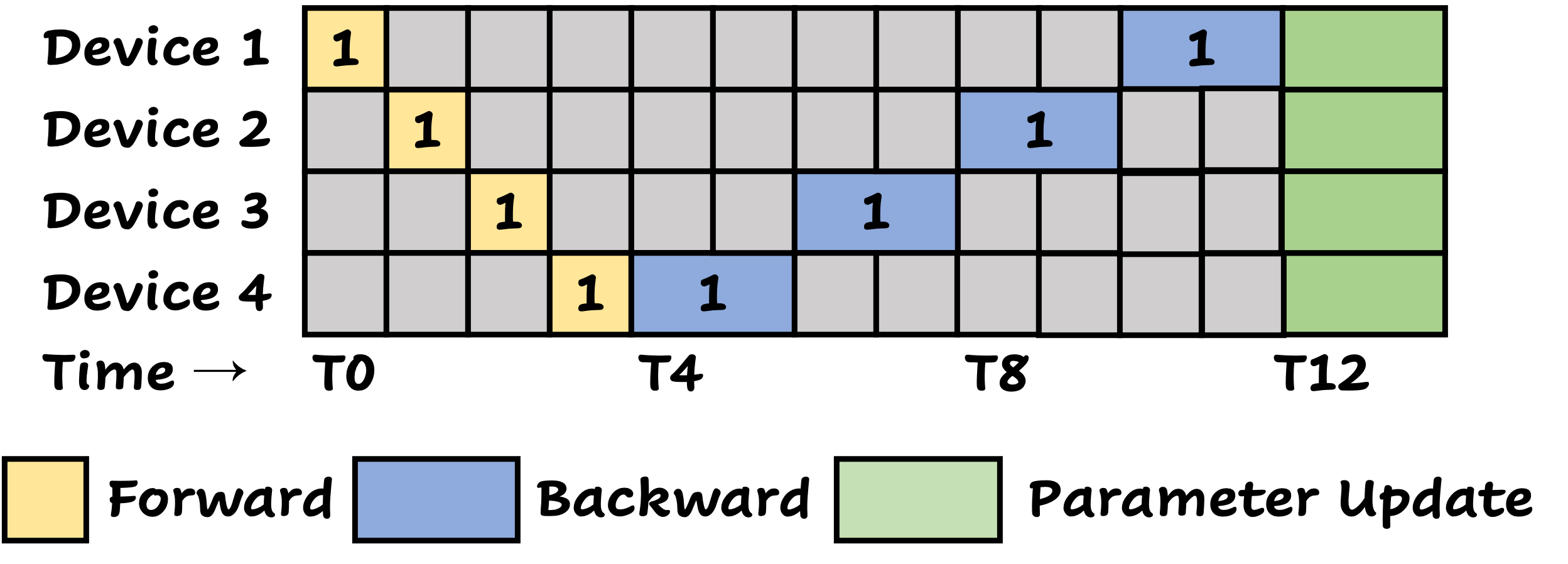
Before implementing this pipeline system, the workflow in each workshop looked like the diagram above. During the first batch’s lifecycle (T1~T4), only one machine was working at a time; when it came time for inspection and parameter feedback (T5~T12), again just one machine was active while the others were idle (gray areas in the figure). Tony quickly spotted the inefficiency: once the first batch moved on to the second stage, the first stage could be processing the second batch, and so on. So the pipeline became:
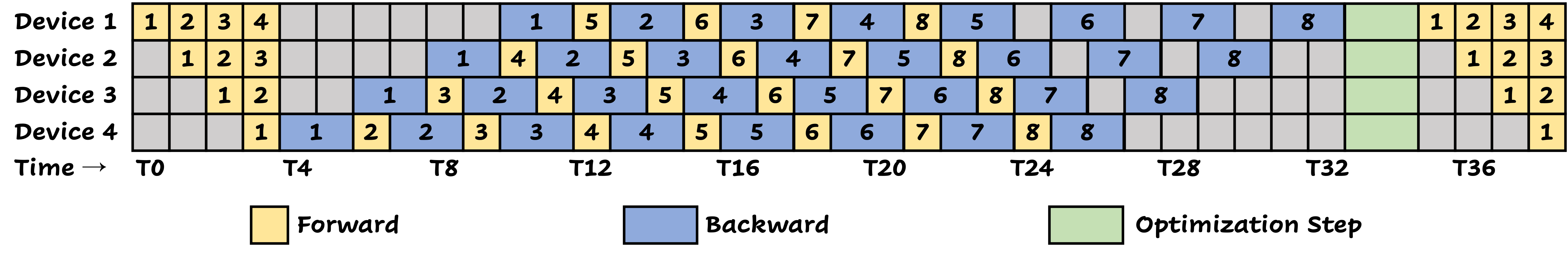
The diagram above illustrates the well-known 1F1B (one-forward-one-backward) pipeline parallelism scheme. Its principle is: whenever a GPU (or a machine) is ready to perform the backward pass on a recent micro-batch, it will prioritize the backward pass. For instance, at time T5, Device 4 must choose between doing a forward pass for the second batch or a backward pass for the first batch, and it prioritizes the backward pass. Meanwhile, all data are backpropagated in micro-batch order; for example, the second micro-batch only starts its backward pass after the first micro-batch’s backward pass has begun. Also, each device keeps a limited number of forward activations (4 in the figure) to avoid storing too many intermediate results for backward computation. Returning to our analogy, these intermediate “activation data” are like the manufacturing logs that the workshop stores to assist with final quality assessment and parameter updates. As you can see, there are still idle periods in the 1F1B pipeline. In large-model training, such idle times are called bubbles—periods when GPUs are waiting rather than working. We aim to reduce these bubbles as much as possible.
After closer observation, Tony discovered that a key source of pipeline “bubbles” was how much time the parameter feedback process took—nearly twice the actual processing time for each batch. That meant once the first stage had processed the fourth batch, it had to wait a long time to receive the feedback updates on the first batch. To address this, he came up with a novel idea: since feedback consumes so much time, split it into two independent parts so they can be decoupled. For example, each process might involve fixture design and manufacturing design. If the fixture design can be updated immediately based on the quality inspection report, independent of the manufacturing design updates, we can eliminate some idle time. Based on this idea, Tony designed the improved pipeline:
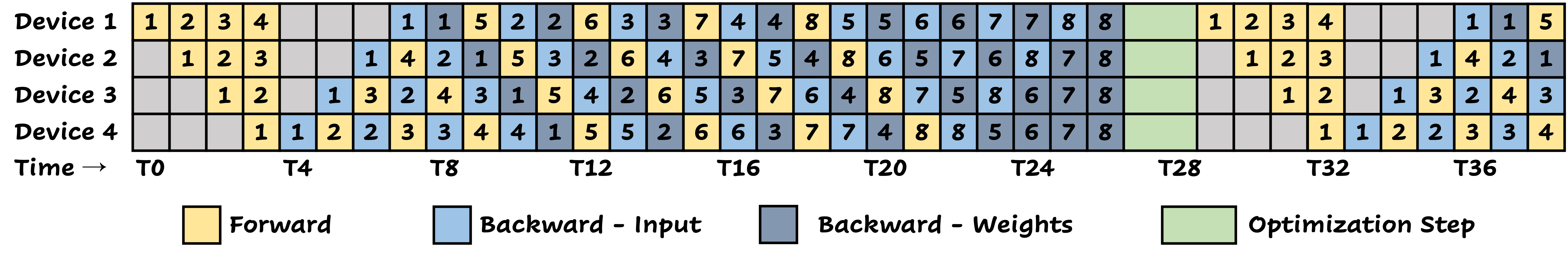
Here, each batch’s feedback is split into two phases: fixture design adjustment (light blue) and manufacturing design adjustment (dark blue). Within the same process stage, there is a dependency among the same feedback phases (e.g., forging’s fixture design must finish before casting can update its fixture design), but different phases don’t depend on each other. This decoupling allows each stage’s fixture design update to be done earlier, while the manufacturing design updates can be delayed, thus reducing idle bubbles compared to the original 1F1B approach.
The scheme above is the ZB1P (Zero Bubble 1F1B) baseline mentioned in the DeepSeek-V3 technical report. It divides the backward pass into two sub-steps in deep learning:
- Input gradient computation: Passing gradients from the current layer back to the previous layer.
- Parameter gradient computation: Computing the parameter gradient for the current layer so it can be updated.
For a linear layer $ \mathbf{y} = \mathbf{W}\mathbf{x} $ with loss $ L $, once we receive $ \frac{\partial L}{\partial \mathbf{y}} $ from the subsequent layer, we need to compute:
- $ \frac{\partial L}{\partial \mathbf{x}} $: to pass the gradient backward to the preceding layer;
- $ \frac{\partial L}{\partial \mathbf{W}} $: for the layer’s own parameter update.
Interestingly, these two computations do not depend on each other in a strict order. Even if a layer has only finished computing (1) but not (2), the gradient can still propagate to the previous layer. Leveraging this fact, ZB1P decouples (1) and (2) so that input gradient (1) can be performed as early as possible while parameter gradient (2) is postponed, thus greatly increasing pipeline scheduling flexibility and efficiency.
By now, you understand the two baseline pipeline schemes in the DeepSeek-V3 report that are compared against DualPipe. Below is a summary table comparing their efficiency:
| Method | Bubble | Activation | ||
|---|---|---|---|---|
| 1F1B | $(PP - 1)(F + B)$ | $1 \times PP$ | ||
| ZB1P | $(PP - 1)(F + B - 2W)$ | $1 \times PP$ | ||
| <!– | DualPipe | $( \frac{PP}{2} - 1) (F\&B + B - 3W)$ | $2 \times PP + 1$ | –> |
Key Parameters:
- $PP$: Pipeline depth, i.e., the number of process stages involved in parallel.
- $F$: Time needed for a forward pass (e.g., each workshop’s initial machining).
- $B$: Time needed for a backward pass (e.g., each workshop’s feedback adjustments).
- $W$: The window size for activation data accumulation—i.e., the upper limit of stored intermediate activations for backprop.
From this table, you can see that ZB1P reduces bubbles substantially compared to 1F1B, at the same level of activation memory usage. By decoupling the backward computations, ZB1P achieves more overlap between forward and backward, thus cutting down idle time. More advanced scheduling strategies (like DualPipe) push this idea further, aiming to maximize resource utilization and parallel performance in large-model training.
In short, Tony’s evolving pipeline schemes—from the original 1F1B to ZB1P and beyond to DualPipe—mirror how large language model training has advanced. Each new innovation reduces bubbles (idle times) and pushes the system to higher performance and better resource utilization.
1.6 When the Pipeline Still Has “Blind Spots”: Limitations of ZB1P
Although ZB1P’s decoupling approach significantly shortens idle periods, Tony’s workshop still experiences some lingering gaps. Imagine a pipeline of Casting → Forging → Heat Treatment → Polishing: once the casting machine finishes its “fixture design update,” it hands that info off to forging, but a deeper stage’s “manufacturing design update” might still have to wait on all preceding updates to be done. Because parts flow through multiple tightly coupled stages, even small delays in one stage can ripple through and create new bubbles.
In large-model training, ZB1P does boost overlap between forward and backward, but it can’t achieve truly simultaneous forward and backward passes. Why?
-
Pipeline bubbles are still present
Traditional pipeline implementations often strictly separate forward and backward: process all micro-batches in forward mode, then do backward. This leads to idle GPUs during each phase. -
Manual scheduling is complex
Conventional pipeline schemes require writing extensive logic: When to send activation tensors? When to receive gradients? If not carefully arranged, you’ll face extra waits or communication bottlenecks. -
Forward and backward can interfere
As more micro-batches accumulate in forward passes, the backward passes can eventually starve the forward pass of GPU resources (e.g., memory or bandwidth). Poor resource management can lead to additional stalls. -
Insufficient front-back overlap
Ideally, we want other micro-batches’ forward passes to run concurrently with backward passes on different GPUs. Doing so, however, requires a sophisticated scheduling design.
Returning to Tony’s workshop example: if both the casting and forging machines are fully utilized at a certain moment, but the heat treatment or polishing machine reduces output for some reason (akin to GPU load imbalance), you may quickly revert to a “front-waits-for-back, back-waits-for-front” scenario. ZB1P already improves scheduling flexibility, but there remain “blind spots” of idle time.
Seeking an even better approach, Tony aimed to further break down the dependencies between forward and backward so they could fully interleave in adjacent pipeline nodes. In other words, if a machine is handling a backward pass, it could still process the next micro-batch’s forward pass. This approach greatly increases pipeline concurrency and minimizes downtime. Tony’s new design for his workshop parallels a new scheduling strategy for model training, called DualPipe, the main focus of this article.
2. DualPipe: A Two-Pronged Pipeline Strategy
2.1 Bidirectional Scheduling: Pushing “Front and Back” onto the Production Line Together
In traditional (single-direction) pipelines such as 1F1B or ZB1P, a machine either performs forward processing or waits for a feedback signal to do backward adjustments. These two modes are usually mutually exclusive. In DualPipe, however, Tony equips each machine with a “timesharing mode” and a flexible front-back transport system that allows the same machine to handle both forward and backward tasks simultaneously. The machine can receive new raw materials from the “front” while also getting a feedback report from the “back.”
By introducing this dual transport system, a machine can keep receiving new parts to process (the forward pass) while at the same time handling the backward pass updates from downstream. In a large language model, this translates to letting forward and backward passes truly occur in parallel, significantly boosting GPU utilization.
Unlike a single-direction pipeline, DualPipe injects micro-batches from both ends of the pipeline. If you picture a linear conveyor belt, previously we only fed data from one side, passing all the way to the end. DualPipe, however, opens up the opposite end as well, so a machine can do forward processing for tasks coming from the left (upstream) while simultaneously receiving backward gradients from the right (downstream). This approach greatly increases overall pipeline efficiency and cuts down idle periods. GPUs can process forward tasks from the “front” and handle backward tasks from the “back” at the same time, thereby avoiding the strict one-way flow that caused waiting times in earlier methods.
Below is a table comparing 1F1B, ZB1P, and DualPipe in terms of pipeline bubbles and activation usage, illustrating how each approach tackles latency and scheduling:
| Method | Bubble | Activation |
|---|---|---|
| 1F1B | $(PP - 1) (F + B)$ | $1 \times PP$ |
| ZB1P | $(PP - 1) (F + B - 2W)$ | $1 \times PP$ |
| DualPipe | $\left(\frac{PP}{2} - 1\right) (F\&B + B - 3W)$ | $2 \times PP + 1$ |
Where:
- $PP$ is pipeline depth (number of pipeline stages),
- $F$ and $B$ are forward and backward times,
- $W$ is the activation window size.
By comparing the three:
-
1F1B
The simplest one-way pipeline. Bubble time is $(PP - 1)(F + B)$. Each stage must wait in a mostly serial fashion. The activation storage is $1 \times PP$. -
ZB1P
By decoupling the backward steps (splitting input gradient and parameter gradient), bubble time shrinks to $(PP - 1)(F + B - 2W)$. Activation usage remains $1 \times PP$. -
DualPipe
Uses a bidirectional pipeline plus overlapping compute and communication to drastically reduce idle times. The bubble time drops further to $\left(\frac{PP}{2} - 1\right) (F\&B + B - 3W)$. However, it demands increased activation storage, up to $2 \times PP + 1$, because each GPU holds extra activation data to support simultaneous forward and backward.
In short, DualPipe trades off a bit more memory usage for a significantly higher overlap between forward and backward, thus achieving greater throughput in large-scale distributed training—just as Tony’s workshop gains higher utilization by letting machines work in both directions simultaneously.
2.2 “Compute-Communication” Overlap Inside the GPU: Doing Calculations While Data Moves
Another key to DualPipe’s efficiency is “chunk-based” or “segmented” transport. In large-scale distributed scenarios, both computation and communication can be major time sinks. If they happen strictly one after another (compute → comm → compute → comm), we’ll inevitably face idle GPU cycles during communication, and idle network bandwidth during compute.
DualPipe splits data transfers into smaller chunks—“micro-batch streaming”—and interleaves them with partial compute tasks, so GPUs can start computing as soon as a portion of the data arrives, rather than waiting for the entire dataset to transfer. Here’s why chunk-based shipping is vital:
2.2.1 Why “Chunked Transport” Improves Efficiency
Imagine Tony’s casting machine has 1,000 parts to send to the forging machine. If we do a one-shot transfer, forging can’t start until all 1,000 are delivered. During that time, forging is idle. After delivery, forging might quickly finish some tasks, only to wait again. This can lead to “you wait for me, I wait for you.”
But if we break the 1,000 parts into several smaller shipments (say 4 or 10 chunks), forging can start working on the first chunk immediately while the second chunk is in transit, removing idle time and ensuring a steady flow of tasks.
In GPUs, this is akin to splitting large tensor transfers or all-to-all communications into smaller pieces, enabling partial results to be computed while the remaining data is still streaming.
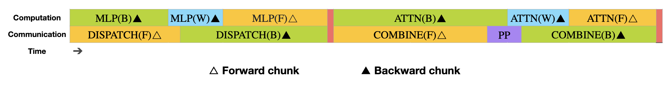
2.2.2 How “Compute-Communication” Overlap Works on GPUs
-
Resource Partitioning
Modern GPUs have multiple SMs (Streaming Multiprocessors). We can allocate some to handle communication (sending/receiving packets) while others handle compute kernels. If communication is chunked into smaller messages, the compute SMs can stay busy while the communication SMs handle the data transfer. -
Fine-Grained Splitting of Tensors
Instead of waiting for the entire model layer’s data to be transferred, we break each layer’s output or gradient into smaller segments. The GPU can compute on the first segment while the next segment is still being transferred. -
Parallel Scheduling
Frameworks like PyTorch support multi-stream asynchronous operations. You issue a communication call (e.g.,cudaMemcpyAsyncor collectives) in one stream while continuing computation in another. You only synchronize when you actually need the results. -
Pipeline Mechanism
As DualPipe introduces bidirectional flow, each GPU both receives data from the previous stage and sends updates to the next stage. By carefully scheduling smaller chunks, communication from “front to back” and from “back to front” can overlap with local compute, forming a tight pipeline across micro-batches and GPUs.
All these enable what we call time overlap between compute and communication—the fundamental reason GPUs don’t sit idle waiting for large transfers to finish.
In a “single-chunk” scenario, you might see:
Time: ======================> Comm: [send all data] -> (wait) -> Compute:[start only after entire data is available]
Resulting in wasted GPU cycles during comm and wasted network bandwidth during compute. By contrast, chunked:
Time:     ==================================>
Info:      [comm chunk1]  [comm chunk2]   ...
Compute:         [compute chunk1]   [compute chunk2]  ...
They overlap like interlocking gears, drastically reducing idle periods and ensuring a continuous workflow. This is how DualPipe sustains high throughput even as model size and parallelism scale up.
Just like Tony’s multi-stage workshop—where partial shipments of parts go back and forth and get processed without waiting for an entire batch to travel—DualPipe leverages chunk-based data flows to keep GPUs near full utilization, effectively hiding communication overhead behind concurrent computation.
3. How the Source Code Implements “Two-Pronged” Parallelism: Key Logic of DualPipe
In the previous section, we used a manufacturing analogy to illustrate how DualPipe enables forward and backward passes to truly run “at the same time” in the same pipeline, thereby maximizing GPU utilization. Here, we’ll explore how DualPipe’s core source code implements these ideas. Specifically, we’ll look at how it handles batch splitting, manages communication, and cleverly interweaves forward-backward tasks to achieve deep overlap and minimal pipeline bubbles.
Note that we won’t parse the code line by line. Rather, we’ll focus on the critical functions and workflows, tying them back to the “machine workshop” analogy to help you understand them more intuitively.
3.1 Basic Class Structure and Initialization
1
2
3
4
5
6
7
8
9
10
11
12
class DualPipe(nn.Module):
    def __init__(
        self,
        modules: Tuple[nn.Module, nn.Module],
        ...
    ) -> None:
        super().__init__()

        ...
        self.module = nn.ModuleList(modules)
        self.overlaped_forward_backward = ...
        ...
modules: This parameter is a tuple of twonn.Moduleinstances, typically representing the “front half” and “back half” of a pipeline. In our mechanical analogy, these could correspond to a combined “forward processing” set of machines (e.g., casting + forging) and another combined set (e.g., quality inspection + parameter adjustment).overlaped_forward_backward: This is a specialized function that checks whether the twoModuleobjects support forward-backward overlap. Only if bothModules implement anoverlaped_forward_backwardmethod (and are of the same type) will the subsequent workflow apply true forward-backward interleaving for the same batch.
Additionally, the code sets up parameters and flags related to distributed training, such as:
self.groupandself.rank: These tie intotorch.distributed, used to manage the pipeline rank (i.e., the stage) of the current process.self.is_first_rank,self.is_last_rank,self.is_in_second_half: Flags that mark whether this node (machine) is at the “left end” or “right end” of the pipeline, i.e., whether it belongs to the first half or the second half.
These flags and mappings resemble the labels Tony might attach to each machine in his workshop, e.g. “Casting Line,” “Polishing Line,” or “Second-to-Last Step.”
3.2 State Management and Reset
Below is the _reset_states method:
1
2
3
4
5
6
7
8
9
10
11
12
13
14
15
16
17
18
def _reset_states(self) -> None:
    WeightGradStore.clear()

    self.input_chunks = ([], [])
    self.output_chunks = ([], [])
    self.input_grad_chunks = ([], [])
    self.output_grad_chunks = ([], [])
    self.labels = None
    self.loss_chunks = []
    self.criterion = None

    ...
    # Various counters for tracking which chunk is being processed
    self.current_f_chunk_id = [0, 0]
    self.current_b_chunk_id = [0, 0]
    ...
    self.comm_ops = []
    self.to_free = []
-
_reset_statesis similar to clearing the workshop and re-laying out tools and logbooks whenever Tony gets a new order:WeightGradStore.clear()removes any stored “parameter gradient” callbacks, preparing for Zero-Bubble or partial-overlap strategies.input_chunks,output_chunks,input_grad_chunks,output_grad_chunks: These are like the “work in progress” parts and their “gradient info.” Initializing them to empty lists so we can fill them with each micro-batch and move them along.- Various counters track the number of forward chunks, backward chunks, send/receive events, etc.
3.3 Forward and Backward Computation: Achieving Overlap on the Same Device
In large-model training, “forward computation” and “backward computation” essentially involve running a forward or backward pass on a tensor and then passing gradients to the previous layer. In the mechanical analogy, forward is “machining the part,” while backward is “checking for defects and adjusting production parameters.” DualPipe wraps these processes in a few methods:
3.3.1 _forward_compute_chunk(self, phase)
1
2
3
4
5
6
7
8
def _forward_compute_chunk(self, phase: int) -> None:
    phase ^= self.is_in_second_half  # dynamically correct the phase
    chunk_id = self.current_f_chunk_id[phase]
    self.current_f_chunk_id[phase] += 1
    inputs = self.input_chunks[phase][chunk_id]
    ...
    outputs = self.module[phase](*inputs)
    ...
- Here, the
phaseis adjusted to choose which sub-module (the “front” vs. the “back” part of the pipeline) is actually used. Then we grab the batch data frominput_chunks[phase]and run forward computation on it. - The resulting
outputswill be stored inself.output_chunks[phase]. - If this is the last stage (
is_last_stage) and acriterionis defined, the “loss” is placed inself.loss_chunks. Think of it as the final workshop outputting a “defect score” for inspection.
3.3.2 _backward_compute_chunk(self, phase, enable_zb: bool = False)
1
2
3
4
5
6
7
8
9
10
11
12
13
14
15
16
17
18
19
20
21
22
def _backward_compute_chunk(self, phase: int, enable_zb: bool = False) -> None:
    if self.forward_only:
        return
    phase ^= self.is_in_second_half
    chunk_id = self.current_b_chunk_id[phase]
    ...
    if is_last_stage:
        # at the last stage, directly call backward on the loss
        loss = self.loss_chunks[chunk_id]
        loss.backward()
        loss.detach_()
    else:
        # run_backward on outputs + output_grads
        outputs = self.output_chunks[phase][chunk_id]
        ...
        run_backward(outputs, output_grads)
    ...
    if enable_zb:
        WeightGradStore.flush()

    # update input_grads
    ...
- For backward, the main logic is: if you’re on the final stage, call
backward()on theloss; otherwise callrun_backward()on the intermediate outputs to pass the gradient upstream. enable_zbactivates the Zero-Bubble (e.g., ZB1P) approach, where some parameter-grad computations are deferred by putting them intoWeightGradStoreand flushing them at the right moment. This aligns with our earlier explanation of decoupling “input gradient calc” and “parameter gradient calc.”- Once backward finishes, the “gradients” for the upstream stage are placed into
self.input_grad_chunks[phase], akin to Tony returning some defect report to the previous machine.
3.3.3 _forward_backward_compute_chunk(self, phase0, phase1)
1
2
3
4
5
6
7
8
9
10
11
12
13
14
15
def _forward_backward_compute_chunk(self, phase0: int, phase1: int) -> None:
    if self.forward_only:
        self._forward_compute_chunk(phase0)
        return

    if not self.overlaped_forward_backward:
        self._forward_compute_chunk(phase0)
        self._backward_compute_chunk(phase1)
        return

    # 1) pre-forward
    # 2) pre-backward
    # 3) overlaped_forward_backward(...)
    # 4) post-forward
    # 5) post-backward
The true core of DualPipe: if overlaped_forward_backward is True, the same GPU can fuse forward and backward for certain batches (like “both hands working together”).
- The function first grabs the forward data from
input_chunksand the backward data fromoutput_chunks, then callsmodule0.overlaped_forward_backward(...).- In the workshop analogy, the operator gathers the new batch of parts to be processed, as well as the defect reports and adjustments from a prior batch, then uses a single “combined machine operation” to handle both forward + backward tasks.
- It finally stores the new output and gradient into
output_chunksandinput_grad_chunks. This means partial forward-backward steps can occur within the same stage, rather than calling them separately or waiting for another stage (as in ZB1P).
3.4 Communication Management: Hiding “Transport Time” Behind Computation
In large-scale model pipeline parallelism, every stage’s GPU frequently needs to communicate with upstream/downstream GPUs (like transporting half-finished parts from casting to forging). DualPipe uses several functions to break down and schedule communication so that computation and communication overlap extensively:
-
_recv_forward(self, phase)/_send_forward(self, phase)
Used to receive/send “forward outputs” or “forward inputs.” In the workshop analogy, handing off the partially processed parts to the next machine. -
_recv_backward(self, phase)/_send_backward(self, phase)
For receiving/sending “backward gradients” or “backward inputs,” analogous to passing inspection reports between machines. -
_commit_and_wait_comm(self)
Internally calls something likedist.batch_isend_irecv(self.comm_ops)to launch all non-blocking communications, thenwait(). This allows compute to proceed in parallel with communication, so the “shipping time” is “hidden” within timeslots when the machine is idle or can devote resources to transfers.
3.5. WeightGradStore: Delayed Gradient Update Design
During backward passes, the same weights may accumulate gradients multiple times. WeightGradStore uses a static queue to hold these updates, then executes them collectively at the right time. Benefits:
- Fewer syncs and memory writes: Instead of updating parameters on every micro-batch, you can batch them up for a single update when appropriate.
- Pipeline integration: Avoid interrupting pipeline concurrency, plus sync at times that overlap with other tasks.
    class WeightGradStore:
        enabled: bool = False
        cache: List[Callable] = []
        funcs_queue = queue.Queue()

        @classmethod
        def put(cls, func: Callable) -> None:
            cls.cache.append(func)

        @classmethod
        def flush(cls) -> None:
            cls.funcs_queue.put(cls.cache)
            cls.cache = []

        @classmethod
        def pop(cls) -> None:
            funcs = cls.funcs_queue.get()
            for func in funcs:
                func()
Note: The
phase ^= self.is_in_second_halftrick is a neat way of “flipping” the phase based on whether the pipeline rank is in the second half, allowing the same function to handle left-to-right and right-to-left data transfers.
3.6 Overall Scheduling: The step(...) Method’s 8 Stages
The core logic resides in step(...). This function is like Tony’s central command that orchestrates all machines. To achieve DualPipe’s two-way pipeline, it proceeds through these phases (in a simplified view, see code comments for details):
-
Step 1: nF0
At pipeline startup, let one end process a certain number of forward batches first. Like partially “pre-processing” raw material on the left side while the right side is idle. -
Step 2: nF0F1
Gradually let the other end begin forward operations so that both directions are activated—calling_forward_chunk(0)and_forward_chunk(1)in alternation. -
Step 3: nB1W1F1
When backward shows up for some batches, mix backward (_backward_chunk(1)) with forward (_forward_chunk(1)), plus_weight_chunk()for delayed weight updates (related to ZeroBubble). -
Step 4: nF0B1F1B0 (main loop)
DualPipe’s main “interleaving” step:_forward_backward_chunk(0,1)/_forward_backward_chunk(1,0)for simultaneous scheduling of forward and backward. -
Step 5: nB1F1B0
Continue driving backward + forward interweaving. -
Step 6: nB1B0
Focus more on backward, lettingWeightGradStoreflush partial gradient data. -
Step 7: nWB0
More “weight update + backward” cycles. -
Step 8: nW
Final weight updates, ensuring all tasks wrap up cleanly.
In the workshop analogy, it’s a “scheduling timetable” with multiple time slots: first let the left-side machines do some initial runs, then after a certain point, the right side also feeds in raw materials; both sides keep passing along half-finished parts and defect reports until everything is done, with a final unify-and-finish step.
The multiple steps may seem complex, but that’s because a two-way pipeline requires careful management of micro-batches at different phases to keep bubbles minimal.
3.7 Summary
From the step(...) orchestration to _forward_backward_compute_chunk(...)’s “fusion of forward and backward,” you can see how DualPipe leverages fine-grained partitioning and two-way injection. On the code side, it greatly hides communication overhead and enables a single GPU to run forward while running backward at just the right times.
Going back to the workshop analogy: a single time slot might see Machine A process new raw materials (forward) while Machine B handles the defect feedback from the previous batch (backward), and the “transport truck” (communication) zips around mostly during those moments of spare capacity—reducing idle time on every machine.
The benefits are evident:
- Minimal pipeline bubbles: DualPipe truly has “front-back concurrency,” lowering serial wait times.
- Extensive communication overlap: Via
_commit_and_wait_comm()and async send/receive, much cross-node all-to-all or pipeline traffic finishes while the GPU is busy computing. - Scalability: Even if the cluster grows (more GPUs, more nodes), as long as compute-comm ratio is managed, this overlap stays effective.
- Memory optimization: Placing the shallowest layer and deepest layer on the same pipeline rank with Zero-Bubble can help reduce middle-layer storage overhead.
Such a “two-pronged” solution significantly speeds up large-model training (e.g., MoE) that demands heavy cross-node expert parallel communication. It can let you train 100-billion-parameter networks on limited GPU resources (like H800s) without grinding to a halt.
4. Conclusion and Outlook
From a machine workshop analogy to large-language-model parallel training, we have covered no parallelism, model parallelism, data parallelism, and pipeline parallelism. In pipeline parallelism, the hardest part is minimizing “pipeline bubbles,” cutting communication wait times, and overlapping forward-backward execution. DualPipe is a high-level solution that cleverly arranges micro-batches and forward-backward timing to reach a “zero-bubble” ideal (or near-ideal), greatly boosting pipeline training speed and utilization.
In short, DualPipe not only conceptually overlaps front and back passes, but also encapsulates communication and scheduling details to let users more easily perform complex pipeline-parallel training. For those wanting to dive deeper into large-model distributed training, studying its source code (plus hands-on testing) can be highly beneficial for developing more efficient parallel solutions.
In a nutshell: like a well-orchestrated assembly workshop, DualPipe synchronizes forward and backward processing to move in tandem, massively improving multi-GPU efficiency and laying a vital technical foundation for the era of large models.
DualPipe 深入浅出:没有分布式训练基础也能看懂的 DualPipe 全方位讲解
过去的一周里,DeepSeek 在社交媒体上宣告这是他们的开源周(OpenSourceWeek),并连续五天放出了多款软件库。前几天分别发布了 FlashMLA(高效 Hopper GPU MLA 解码核)、DeepEP(面向 MoE 的专家并行通信库)以及 DeepGEMM(支持 FP8 的 GEMM 库)。而就在第 4 天,他们一口气开源了三大组件:DualPipe、EPLB 以及 profile-data,其中的 DualPipe 因为引入了“双向流水线并行”这一核心理念,引起了广泛讨论。
这篇博客将聚焦于 DualPipe 的核心思路:如何在大模型的训练阶段,实现前向(forward)与后向(backward)的完全重叠,从而大幅降低流水线中的「空闲时间(bubble)」。为了让读者们更好地理解这些概念,本文从一个通俗易懂的类比——“机械加工中的工艺优化”——切入,并在每个部分先讲清楚比喻场景,再与深度学习中的并行训练一一对应,让读者可以在脑海中形成清晰的“具象”画面。同时,文末我们将深入到 DualPipe 技术的源码层面,探讨它如何进一步减少流水线气泡、实现前后向交叠、将通信带来的压力减小到极致,且如何在较复杂的混合并行场景下落地。
1. 引言
在大语言模型(Large Language Model)如 GPT-3、PaLM、LLama 等火热的当下,分布式训练已成为突破单卡 GPU 极限、成功训练超大模型的必备手段。我们经常听到诸如“数据并行”“模型并行”“流水线并行”等名词,但对初学者来说,很难直观把握它们之间的区别与联系。尤其是当大家阅读到一些高级用法,如 DeepSeek-V3 里采用的 DualPipe 技术,可能会觉得晦涩难懂。
与此同时,在工业领域,优化生产工艺需要经过无数次试错;在人工智能领域,训练大语言模型同样需要反复调整参数。这两件事看似毫不相关,却有着惊人的相似性。让我们跟随老王机械加工厂的故事,看看如何用车间里的机床与工序,理解大模型训练中的四大并行技术。
1.1 单卡时代:从手工小作坊说起
在苏州工业园区,老王拥有一个不大不小的机械公司,他的公司的主要业务是为机械产品的优化加工工艺,比如铸造温度、淬火时间、切削角度等等。每当一个新的订单到来时,老王会根据经验设计一份初始工艺手册,按照这个工艺手册进行加工,对加工后的零件进行质量检测,并根据当前加工出来的零件缺陷,从后往前,对每一道工艺进行参数调整:比如当前加工出来的产品有空隙缺陷,就告诉我们铸造温度应该升高一些。
老王的工艺流程其实和大模型训练非常契合:所谓的工艺手册就像大模型的参数一样、而加工的零件就是大模型的训练数据、不同的工艺对应大模型的各种层,机床就像 GPU 一样,最后所谓的质量检测就是损失函数的计算、而根据之间结果对工艺进行调整也正是大模型的梯度回传和参数更新的过程。
在创业初期,老王最初只接螺丝钉加工订单。这类零件加工简单,只需在一台多功能机床上完成切削、打磨两道工序。每当出现次品,老师傅就会对着成品倒推问题:如果是打磨不匀,就调整打磨参数;若是切削误差,就修改刀具角度。整个过程都在同一台机床上闭环完成。老王的工厂就像一个手工小作坊:不成体系不成规模,但对于简单的零件还是够用的。
这就像单GPU训练场景。模型的所有层(工序)都在同一块GPU(机床)上顺序执行,前向传播(加工零件)和反向传播(参数调整)都在单一设备内完成。虽然简单可靠,但面对复杂任务时,设备性能就会成为瓶颈。
1.2 模型并行(Model Parallelism):工艺手册的拆分艺术
有一天老王接到了一个以前没有遇到过的大单子:发动机曲轴的工艺优化,老王发现自己的单台机床根本无法胜任这个工作。他将铸造、热处理、精密加工等工序拆分到三台专业机床上。每台机床的操作手册都只记录对应工序的参数标准,且调整铸造参数时必须同步考虑对后续工序的影响。此时,老王发现了一个以前没有遇到过的问题:机床的闲置问题。在零件进行铸造阶段,热处理和精密加工的机床好像没有事做;于此同时,把一个机床的加工结果搬运到另一个机床上加工的过程好像也需要时间,而在“搬运”的过程中如果不做合理的安排可能会使机床闲置的问题更加严重。
在大语言模型中,这对应“模型并行”(Model Parallel)。当模型的体量过大,单个 GPU 无法容纳所有参数时,就把模型本身(如不同层、不同模块)拆分到多个 GPU 上。在上边的例子中,铸造就像是模型的输入层、热处理是中间层、而精密加工是输出层。模型训练时每个GPU负责特定层的计算,必须通过设备间通信传递中间结果。这种方法的代价是不可避免的 GPU 闲置以及需要频繁的跨设备数据传输。老王遇到的问题正是 GPU 之间的调度和通信的问题。
1.3 数据并行 (Data Parallelism):克隆车间计划
为加速工艺参数优化,资金充裕的老王在隔壁建了三个完全相同的车间。每个车间都配备全套四条产线,分别加工不同批次的涡轮盘(数据分片)。收工时,四个车间的工艺主任会开会比对数据,统一修订工艺标准。原本收到的 10,000 块原材料加工优化需要一个月,现在只需要半个月了。老王很好奇,为什么我的车间数量翻了四倍,而速度只提升了两倍呢?和车间主任们沟通了解到,原来虽然工艺相同,不同的原材料在加工的过程中会遇到一些独特的问题,导致四个车间的收工时间不一样,你等等我、我等等你,时间就这么被浪费了。
这对应“数据并行”(Data Parallel)。每个车间(GPU)都持有完整的工艺手册(模型参数副本),但加工不同的原材料批次(数据分片)。当遇到次品(计算损失)时,各车间独立推导本批次的工艺调整方案(本地梯度),但需要将所有调整方案汇总平均(All-Reduce)后,才能更新统一的工艺标准(全局参数)。这种方法的瓶颈在于:最慢的车间(straggler GPU)会拖累整体会议进度(通信同步开销),且车间间的沟通耗时(All-Reduce带宽)随着车间数量增加而显著上升。
1.4 张量并行(Tensor Parallelism):协作加工超大单件
有一天老王出息了,接到了一个超级订单:飞机机体制造的工艺优化。这种订单加工的零件本身极其巨大,比如飞机机翼。尽管机翼只是某一道工序里的一个大部件,但仍然需要调用很多台同样的机床进行协同。也就是说,这个单件虽然属于某个特定的工序模块,但其体量依然超出了单台机床的处理能力。因此,老王就安排多台相同功能的机床一同来完成同一个大零件的加工。
在大语言模型训练中,这对应“张量并行”(Tensor Parallel)。即便将模型分割成不同模块后,某些单个模块本身依然很大。此时,需要把这部分网络层对应的张量再进行更细粒度地拆分,分别放到多个 GPU 进行并行计算。比如把一个巨大的矩阵分割成不同的块,分别放到不同 GPU 上并行做矩阵乘法,再把结果合并。这样,单层的计算负载也能够通过多卡来分摊。
这时,老王发现对机床的调度已经成了提升他工作效率的重中之重,因为此时不同机床间的协作非常密切,大部分机床都只负责某一部分或者某一小部分的零件加工,零件需要频繁地运送到某个机床又运送出去,后边工序的机床必须要前一个工序结束后才能工作,在质检后的反馈阶段,前一个工序的参数调整又必须等待后一个工序的参数调整完毕。这样就留下了大量的闲置问题:同时加工同一个零件的机床在等着他的兄弟机床结束任务、后一个机床在等前一个机床的工件送过来,又或是前一个机床在等后一个机床的反馈报告。老王觉得必须做点什么才能让自己公司的效率更高了。
这对应”张量并行”(Tensor Parallel)的深层逻辑。当单个工序(模型层)的处理需求超过单台机床(GPU)的承载能力时,就需要将巨型零件(大张量)拆分为多个部件,分发给相同功能的机床组(GPU组)协同加工。比如机翼的抛光工序需要四台机床分别处理不同区域的表面,再通过拼接(张量通信)确保接缝处的完美衔接。但这类协作带来了三重挑战:零件拆分/组装需要额外运输时间(张量切分与合并的通信开销)、任何机床的延迟都会拖慢整组进度(同步等待)、质检反馈需要在机床组内部完成多轮协商(梯度同步),这些因素共同导致了新的闲置形态——”协作气泡”。
1.5 流水线并行 (Pipeline Parallelization):让不同机床同时高效运转
针对不同工序间的协作困境,老王设计了一套精巧的流水线系统:如果原始的加工路线是:铸造 - 锻造 - 热处理 - 抛光,当铸造机床完成第一批零件的初加工时,这批零件立即被送往锻造,而此时铸造机床已开始处理第二批零件;当第一批零件完成锻造进入热处理线时,第二批零件恰好在锻造线就位——就像多米诺骨牌般环环相扣。
具体得讲,在未实行流水线系统之前,四个车间的工作模式就像上图展示的这样,第一批原料在被加工成成品等待检验前(T1~T4),每个时刻仅有一台机床在工作,而当质检报告生成后,参数调整又按顺序原路返回,导致在参数调整阶段(T5-T12),仍然只有一台设备没有处于闲置状态。在上图汇总,灰色区域表示在对应时间段,该车间处于闲置状态。聪明的老王一眼就看出来问题:在第一批原料送给第二道工序的时候,第一道工序完全可以运送第二批原料了,同理,在第一批原料送给第三道工序的时候,第二批原来也送到了第二道工序,此时第一道工序已经开始进入第三批原料了。如此一来,这个生产线路就变成了下边这个样子:
上图展示的正是著名的 1F1B(one-forward-one-backward)流水线并行方案。其基本原则是:当某个 GPU(或机床)发现可对最近一批数据执行梯度回传时,便优先进行后向传播。例如,在 T5 时刻,Device 4 面临两个选择——要么开始执行第二批数据的前向传播,要么对第一批数据进行后向传播;按照规则,它会优先处理第一批数据的后向传播。与此同时,所有数据均按批次顺序依次回传,后续批次的后向传播永远在前一批次的后向传播全部启动后才开始。此外,每个设备在前向传播过程中最多只能累积一定数量的激活数据(在图中为 4),以确保每次前向计算保存的中间数据(activation)足以支撑后续的梯度回传,回到我们的例子,就好像机械加工的过程中记录的中间数据,都是在质检报告生成后用于辅助判断工艺参数调整的重要数据。举例来说,在 T5 时刻,GPU 1 虽有机会处理第五批数据的前向传播,但为了避免激活数据过多而影响后向传播所需的存储和效率,它选择不再累积新的前向任务。显然,即使在 1F1B 流水线方案下,部分设备仍可能出现短暂的闲置状态——这就是我们在大语言模型训练中所称的“气泡”。气泡的存在意味着设备资源没有被充分利用,降低了整体训练效率,而这正是我们迫切希望通过更先进的调度策略来解决的问题。
为了进一步优化流水线调度,老王对整个过程进行了深入观察,发现气泡较大的根本原因在于各车间组织质检报告与参数调整的反馈时间过长——对一批材料进行反馈调整的耗时大约是该批加工时间的两倍。这导致第一道工序在加工完第四批材料后,必须长时间等待才能完成第一批数据的反馈调整。为此,老王提出了一个开创性的思路:既然反馈过程耗时如此,不妨将其拆分为两个独立部分,实现解耦。比如,每一道工艺可能同时涉及夹具设计和加工方案设计;如果每台机床能先根据质检报告对夹具设计进行参数调整,再对加工方案进行调整,而这两者又相互独立(即上一工序的夹具调整无需等待当前工序的加工方案反馈),则整体气泡率便能大幅降低。基于这一理念,老王设计了如下图所示的改进版流水线系统:
在该设计中,每批材料的参数调整被分为两步——浅蓝色代表夹具设计调整,深蓝色代表加工方案调整。在同一工序中,同一步骤的参数调整存在依赖关系(例如,在铸造-锻造-热处理-抛光的流程中,只有当锻造工艺的夹具设计完成后,铸造工艺才能启动对应的调整);而不同步骤之间则相互独立(例如,锻造工艺的夹具设计调整无需等待抛光工艺的加工方案反馈)。因此,与最初的 1F1B 方案相比,该设计在保证相同激活数据数量(图中为 4)的前提下,有效减少了气泡的数量。
上图所示正是 DeepSeek-V3 技术报告中,与 DualPipe 进行比较时采用的第二个基线——ZB1P 方案。上图就是在 DeepSeek-V3 技术报告中,和 DualPipe 做比较的第二个基线:ZB1P,他在保证了和 1F1B 相同 activation 数量的情况下(图中是4)进一步得减少了 bubble 的数量。在大语言模型训练中,梯度回传通常分为两大步骤:
输入梯度计算:将梯度从当前层传递至上一层;
参数梯度计算:计算当前层参数的梯度以便更新。
以一个线性层为例,其前向计算为 $\mathbf{y} = \mathbf{Wx}$,当损失 $L$ 传回时,我们获得 $\frac{\partial L}{\partial \mathbf{y}}$;接着需计算两个梯度:(1) $\frac{\partial L}{\partial \mathbf{x}}$ —— 用于梯度回传至上一层;(2) $\frac{\partial L}{\partial \mathbf{W}}$ —— 用于当前层参数更新。令人有趣的是,这两项计算在逻辑上并不直接相关:即便某层只完成了 (1) 而暂未执行 (2),梯度依然能够自然地向上回传。正是基于这一特性,ZB1P 方案将每一层的 (1) 与 (2) 解耦,使得输入梯度的回传(1)能够提前完成,而参数梯度的计算(2)则可以稍后启动,从而大幅提升了流水线的调度自由度和整体效率。
现在,你已经全面了解了 DeepSeek-V3 技术报告中与 DualPipe 比较的两种流水线并行算法的原理。报告中还提供了下表,对不同流水线并行算法的效率进行了量化比较:
| Method | Bubble | Activation |
|---|---|---|
| 1F1B | $(𝑃𝑃 − 1) (𝐹 + 𝐵)$ | $1 \times 𝑃𝑃$ |
| ZB1P | $(𝑃𝑃 − 1) (𝐹 + 𝐵 - 2W)$ | $1 \times 𝑃𝑃$ |
核心参数说明:
- $𝑃𝑃$ :流水线深度,即参与并行计算的工序数量;
- $𝐹$ :前向传播所需时间,对应各工序进行初步加工的时长;
- $𝐵$ :后向传播所需时间,对应各工序完成反馈调整的时长;
- $𝑊$ :激活数据累积窗口大小,即在梯度回传过程中用于保存中间激活数据的上限。
从上表可以看出,ZB1P 方案在保持与 1F1B 相同激活数据数量的前提下,通过将梯度回传过程拆分并解耦,显著降低了气泡数量,从而缩短了设备等待时间,提升了整体训练效率。更先进的调度策略(如 DualPipe)正是在这一优化思路基础上进一步拓展,致力于最大限度地提高大模型训练时的资源利用率和并行性能。
综上所述,老王通过不断优化流水线调度策略——从最初的 1F1B,到改进后的 ZB1P,再到最新的 DualPipe 技术——正如大语言模型训练中的不断演进与突破,每一次创新都在减少“气泡”对整体效率的影响,推动着系统向更高的性能和更优的资源利用率迈进。
1.6 当流水线依然有“死角”:ZB1P 的局限性
虽然 ZB1P 的解耦思路有效地缩短了气泡,但在老王的机床车间中,仍然存在一些“死角”式的空闲时间。试想一下:在铸造 - 锻造 - 热处理 - 抛光这个工艺路线中,老王的铸造机床刚完成了某批材料的「夹具设计调整」就将夹具参数交给下一道锻造工序,但此时后面某道工序的“加工方案调整”却无法立刻开始,因为它依赖于前一步骤的全部调整完成后才会逐层传递下来。由于零件的流动和多道工序的耦合关系依旧较紧密,一旦中间某道工艺的加工速度出现轻微延迟,就可能再次在流水线中累积出空闲时间,形成新的“气泡”。
在大模型训练中,ZB1P 方案虽然将输入梯度与参数梯度进行了解耦,让前向与后向的 overlap(重叠)程度比 1F1B 高出了不少,但依旧无法达到“前向与后向完美并行”这一理想状态。原因在于:
- 流水线气泡仍然存在
在以往的实现中,前向和后向是两个完全分开的阶段:先把所有微批数据完成前向,再做后向。这样一来,后传阶段就会浪费前面机床资源,气泡现象严重。 - 手工调度复杂
常规的流水线并行实现,需要手动编写大量的逻辑,比如在第几个微批的哪个时刻去发送激活值?什么时候再接收梯度?每个阶段如果不精心安排,整体就会出现等待或通信瓶颈。 - 前后相互挤压 前向传播虽然先行一步,但当批次数量非常大、模型层数较多时,后向计算启动多轮后,可能“挤占”前向计算所需的硬件资源(例如显存、带宽等);若资源管理不当,也会引发意外的等待和空闲。
- 缺少前后向交叠
在深度学习里,如果能让后向计算和前向计算(针对其他微批次)同时在不同 GPU 上并行,就能极大地提高利用率。然而,手动实现这套逻辑往往很繁琐。
拿回到老王的机床车间举例:当铸造机床与锻造机床在同一时刻几乎满载工作时,热处理机床或抛光机床一旦因为某个机械故障(类似于 GPU 运算负载不均)而被迫降低产能,那么整个流水线又会变得“前等后、后等前”。尽管 ZB1P 已经让调度灵活了不少,但这种多机床、多道工艺串行协作的空闲死角仍然无法完全避免。
于是,老王又琢磨出了更新的升级方案——通过更深层次地“打散”前向与后向的依赖,让两者在同一流水线的相邻节点中能够充分地相互交错与重叠。换句话说,假如能让各个机床在处理后向时,依然能接收甚至处理下一批次或下一道工序的前向任务,那么流水线的并行度便能进一步加大,从而将空闲时间压缩得更小。基于这种思路,老王开发出了一个在模型训练中同样适用的新调度策略,也就是本文的重点——DualPipe。接下来,我们将从高层视角介绍 DualPipe 的核心思想。
2. 双管齐下的流水线调度:DualPipe
2.1 双向调度(Bidirectional Scheduling):把“前后”同时推上生产线
在传统的流水线(即单向流水线)中,如1F1B 或 ZB1P,一台机床要么处于“前向加工”状态,要么被动等待上游机床的反馈信息以进行“后向调整”,二者通常是互斥的。在 DualPipe 中,老王为机床配备了一个“分时工作模式”和“灵活的前后道信息传输系统”,让同一台机床可以同时进行前向和后向的操作:一方面可以执行原材料的加工任务,同时可以接受从后方传递过来的质检报告并对当前站点进行对应的参数调整。有了这个双向运输系统,一个机床在同一时刻可以不断地接收从上游送来的原材料(对应前向输入)和从下游传来的成品反馈(对应后向梯度),真正做到“双管齐下”。
这么做有什么好处呢?DualPipe 的出现,正是为了让流水线里的前向与后向能真正做到同时进行,在大语言模型的训练当中,这么做可以最大限度地利用 GPU 资源。和传统的“单向流水线”不同,DualPipe 允许从流水线的两端同时注入微批次(Micro-batches)。如果把流水线想象成一个长长的传送带,过去我们只能从传送带的一头放入原材料、依次通过多台机床到达终点;而 DualPipe 则在“传送带的左端和右端”同时进行传输,让机床既能对“左端”(上游)送来的原材料进行前向加工,又能在稍后对“右端”(下游)送来的半成品进行后向调整。这个做法极大地提升了流水线整体的利用率,使得 GPU 既能处理来自“前段”的前向任务,也能接收“后段”的反馈并执行部分后向计算,避免了单向流动带来的等待。
下面这个表展示了三种流水线调度方案在“气泡”(Bubble)和激活数据(Activation)方面的差异,直观地反映了不同方法在隐藏通信延迟与调度资源方面的成效:
| Method | Bubble | Activation |
|---|---|---|
| 1F1B | $(𝑃𝑃 − 1) (𝐹 + 𝐵)$ | $1 \times 𝑃𝑃$ |
| ZB1P | $(𝑃𝑃 − 1) (𝐹 + 𝐵 - 2W)$ | $1 \times 𝑃𝑃$ |
| DualPipe | $( \frac{PP}{2} − 1) (𝐹\&𝐵 + 𝐵 − 3𝑊)$ | $2 \times 𝑃𝑃 + 1$ |
其中,$𝑃𝑃$ 表示流水线的深度,即参与计算的阶段数;$𝐹$ 和 $𝐵$ 分别代表前向与后向计算所需的时间,而 $𝑊$ 则是激活数据累积的窗口大小。
通过对比三个方法,我们发现:
-
1F1B 方法: 这种最基础的单向流水线调度方式,其气泡数量为 $(𝑃𝑃 − 1)(𝐹 + 𝐵)$。也就是说,每个阶段在前向和后向之间都有固定的等待时间,整个流水线几乎是严格串行的。激活数据则为 $1 \times 𝑃𝑃$,说明每个流水线阶段仅需存储一份激活数据。
-
ZB1P 方法: 通过将后向传播的部分计算(例如输入梯度与权重梯度的拆分)解耦,ZB1P 成功减少了气泡数量,将其降低到 $(𝑃𝑃 − 1)(𝐹 + 𝐵 - 2𝑊)$。不过,激活数据的需求并未改变,仍然是 $1 \times 𝑃𝑃$。
-
DualPipe 方法: DualPipe 采用双向流水线和计算与通信重叠的策略,将前向和后向同时注入流水线,从而大幅度降低了流水线中的空闲等待(气泡)。表中显示,其气泡数量为 $(\frac{𝑃𝑃}{2} − 1)(𝐹\&𝐵 + 𝐵 − 3𝑊)$。可以看到,相较于传统方法,气泡数明显减少,但为实现这种重叠调度,激活数据的存储需求相应提升到了 $2 \times 𝑃𝑃 + 1$。
通过这个表格,我们可以直观地看到 DualPipe 在调度上所作的优化:
- 气泡减少:双向调度和通信重叠使得前向和后向可以并行进行,从而减少了等待时间;
- 激活数据增加:为了支持这种高效的重叠机制,需要在每个 GPU 上额外保留一份激活数据,从而使得激活存储量比传统方案略有增加。 换句话说,DualPipe 是在“牺牲”少量显存的前提下,极大地提高了流水线的利用率,使得 GPU 在大规模分布式训练中能以更高的吞吐率持续运转。这正如老王在车间里通过引入双向运输系统,不仅提高了机床的利用率,还确保了在高负载下依然能保持稳定高效的生产。
2.2 GPU 里的“计算-通信”交错:实现“边运边算”
“分段运输”是 DualPipe 将 GPU 的运算潜力挖掘到极致的另一大杀器。那么,为什么分段运输这么重要呢?在大规模分布式训练中,“计算”和“通信”往往是两大耗时主力。如果它们都按照“整块、顺序”来执行,就会变成:先等通信把整个数据从上一台 GPU(或机床)传完,再进行计算;计算完成后,再一次性把下一批数据传过来……周而复始。这样一来,等待是不可避免的:在通信时计算资源闲置,在计算时网络资源又闲置。
DualPipe 之所以要把大块通信“拆分”成若干个小段(我们可以称之为“小份运输”),并在每一小段传输过程中穿插一部分计算,核心目的就是让 GPU 不必傻等所有数据都到齐才能开始工作。下面通过一个更具体的比喻和技术逻辑,来解释为啥这样做能“边运输、边加工”,从而减少(甚至隐藏)通信带来的空闲时间。
为什么“分段运输”更高效
设想老王有一台“铸造机床”要把一车零件(比如 1000 个)运送给下一台“锻造机床”做下一步加工。如果采用“整批一次性运输”——也就是等到把全部 1000 个零件搬运过去之后,锻造机床才能开始干活。那么:
- 在运送的那段时间里,锻造机床一直处于无事可做(idle)的状态;
- 铸造机床送完这 1000 个零件后,还要额外等待一下,看看锻造机床是否能及时消化完;
- 如果锻造机床处理速度比运输速度快或慢,两边都容易形成 “你等我、我等你” 的浪费。
分段运输的思路: 若把这 1000 个零件拆成 4 次或 10 次小批量运输,只要第一批货物到达锻造机床,这台机床马上就能动工对前几百个零件进行锻造;与此同时,铸造机床(或搬运车)可以继续把第二批、第三批、第四批材料在后台运过来。
- 对锻造机床来说,它不用等所有材料都送达才能开工;它开始锻造第一批的同时,后几批尚在运输。
- 搬运车(通信)也不需要等待锻造机床“空出来”再去送下一批,而是能根据状态继续分段运输。
- 等到锻造机床处理完第一批零件之际,第二批零件可能也刚好运达,机床可以紧接着锻造第二批,如此交替推进,几乎没有空闲。
核心逻辑是:只要我们把大批量的工作“分块”(或称“流水化”),就能让计算和通信在时间上相互穿插。通信并非一次性把所有东西运来,而是一段段地送;计算也不用一直等到全部数据到齐才执行,而是收到一点就先干一点。双方像齿轮一样咬合在一起,从而把可能的等待时间“压缩”到最小。
GPU 里的“计算-通信”交错:如何实现“边运边算”
把这个思路放到 GPU(尤其是多 GPU、跨节点)环境下,具体会涉及几点:
-
在计算和通信之间进行资源划分 GPU 有多个 SM(Streaming Multiprocessors)。当我们做大规模 all-to-all 或者 pipeline 传输时,可以让部分 SM 负责发包/收包(通信),另一些 SM 或流 (Stream) 负责进行前向或后向计算。只要通信包不是太大,或者被拆分成较多小包,那些专门负责计算的 SM 就可以在“通信流”干活时依然执行算子,不用整块阻塞。
-
数据按微批次或更小块切割 比如有一个模型的若干个层的特征张量需要传输,DualPipe 并不会一次性把这几个层全部发完再进行算子计算,而是分成若干小块(如甚至拆分到某个 attention 模块这种粒度)。GPU 只要收到第一小块数据,就可以在计算流中先启动一部分前向或后向运算。这样就像“先送两箱货,机床马上开工;后面继续分批往下送”。
-
通信与计算的并行调度 在 PyTorch 里,cuda 提供多流(multi-stream)异步执行:发起通信 (P2P ops, all-to-all ops) 后,程序无需立刻 wait(),可以让计算流直接开始干别的活。只有在真的需要用到通信结果的那一刻,才去等待对应的事件。就像老王给搬运车下达运输命令(异步通信)之后,机床就去干别的事情,直到下一批材料实际用得到的时候,才会等待搬运车把货送达。这就是“在运输过程中穿插加工计算”的本质:发起运输命令后,立刻让 GPU 去计算之前已经到达的那部分数据,而不是卡在那边干等传输结束。
-
流水线机制 考虑到上边提到的 DualPipe 额外加入的双向流水线的思路,让当前 GPU 既能等待来自“前面的输出”,也能把后向的梯度送往“前面的 GPU”。在宏观调度上,多个微批次与多个 GPU 形成一个环环相扣的管线,一边发送数据,一边接受下一部分数据,并行执行。
为什么能避免闲置?根本是“时间重叠”与“分块解耦”
最终,我们把“整块”的通信和计算分解成多次小规模的交替操作。从时间线上来看,通信和计算往往呈下列交叉图案:
时间轴:  ==================================>
通信流:   [comm chunk1]  [comm chunk2]   ...
计算流:         [compute chunk1]   [compute chunk2]  ...
- 当
comm chunk2开始发送时,compute chunk1可能已经在算前向/后向了; - 当
compute chunk2需要数据时,comm chunk2大概率已快传完了; - 双方就像齿轮一样咬合,不会出现长时间空转。
如果是大块整体传输,则类似:
(整块通信) [comm all data] (等待结束) -> [compute all data]
- 计算必须等通信完全结束才能开始,通信完成后又可能很快结束,导致通信通道闲置;
- 期间 GPU 做不了别的事情——浪费了大量潜在计算时间。
也就是说,通过分块 + 并行调度,我们让通信过程与计算过程在时间线上尽量重叠(overlap),于是之前被浪费的空闲时段被“填补”了。当通信在进行时,计算也在进行;当计算需要更多数据时,新一批数据往往已经在路上或已送达。
正因为此,DualPipe 在模型规模“爆炸式”增长、并行度加大时,依然能保持较高的吞吐率。因为即使通信时长在增大,只要管理好分配给通信的 GPU SM 资源比例,就可以将大部分通信操作隐藏到并发的计算中。这与流水线工厂在接单量暴增时,只要车间产线设置得好,运输环节和工艺环节两条线“各司其职、相互交错”,就能稳定地“吃下”更多订单并保证整体效率。
3. 源码如何实现“双管齐下”:DualPipe 关键逻辑解析
在上一个章节里,我们用机械加工的类比方式,说明了 DualPipe 如何让前向 (Forward) 和后向 (Backward) 真正地在同一个流水线上“同时上阵”,以最大化地利用 GPU 资源。下面,我们来看看 DualPipe 的核心源码如何将这一思路落到实处,并通过拆分批次、管理通信、以及巧妙调用“前向-后向”协同来实现高度的重叠和极小化的流水线气泡。
本文不会按行解析,而是通过重点函数与流程的视角进行剖析,并与之前的“机床车间”类比相呼应,帮助你更好地理解。
3.1 类的基本结构与初始化
class DualPipe(nn.Module):
    def __init__(
        self,
        modules: Tuple[nn.Module, nn.Module],
        ...
    ) -> None:
        super().__init__()

        ...
        self.module = nn.ModuleList(modules)
        self.overlaped_forward_backward = ...
        ...
modules:这里传入的是两个nn.Module的元组,通常代表流水线的“前半段”和“后半段”。想象一下,在机械加工的流水线里,这可能对应“前向加工”的组合机床(如铸造+锻造)和“后向调整”的另一个组合机床(如质量检测+参数调整)。overlaped_forward_backward:用于判断这两个Module是否支持前后向重叠的专用函数。只有当传入的Module有overlaped_forward_backward这个方法(且类型相同),才会在后续流程里真正地进行前后向同一批次的紧密交织。
与此同时,代码中还设置了一系列与分布式训练流程相关的参数和标记,如:
self.group和self.rank:与torch.distributed相关,用于管理当前节点在流水线中的PP Rank(哪个阶段)。self.is_first_rank,self.is_last_rank,self.is_in_second_half:标记当前节点(机床)在“流水线”中的位置,是在“左端”还是在“右端”、是前半段还是后半段。
这些标志位和映射表,类似于老王在车间里给每台机床贴上的“这是铸造线”“这是抛光线”“这是倒数第二工序”等标签。
3.2 状态管理与重置
_reset_states 方法
def _reset_states(self) -> None:
    WeightGradStore.clear()

    self.input_chunks = ([], [])
    self.output_chunks = ([], [])
    self.input_grad_chunks = ([], [])
    self.output_grad_chunks = ([], [])
    self.labels = None
    self.loss_chunks = []
    self.criterion = None

    ...
    # 各种计数器,用于追踪当前处理到第几个 chunk
    self.current_f_chunk_id = [0, 0]
    self.current_b_chunk_id = [0, 0]
    ...
    self.comm_ops = []
    self.to_free = []
-
_reset_states就像每次老王接到新订单之前都会清空生产线、重新摆放刀具和记录簿一样: WeightGradStore.clear():将之前存储的需要延迟执行的“参数梯度计算”回调函数全清空,为后续的 Zero-Bubble 或部分重叠做准备。input_chunks,output_chunks,input_grad_chunks,output_grad_chunks:相当于流水线里的“在制品”和它们的“梯度信息”。初始化为空的列表是为了逐步把每一批(micro-batch)塞进来再往后传。- 一系列计数器:用来跟踪当前处理到第几个前向批次、第几个后向批次,或者是已经发送/接收了多少次数据等。
3.3 前向与后向计算:如何在同一设备上实现交叠
在大模型训练里,“前向计算”与“后向计算”的核心逻辑大多是对张量执行一次前传或后传,然后将梯度往上一层传递。对于机械类比而言,前向就像“对零件进行加工”,后向就像“对零件的质量缺陷进行追溯并调整生产参数”。DualPipe 里分别封装了下面这些方法来完成这个过程:
3.3.1 _forward_compute_chunk(self, phase)
def _forward_compute_chunk(self, phase: int) -> None:
    phase ^= self.is_in_second_half  # 动态修正 phase
    chunk_id = self.current_f_chunk_id[phase]
    self.current_f_chunk_id[phase] += 1
    inputs = self.input_chunks[phase][chunk_id]
    ...
    outputs = self.module[phase](*inputs)
    ...
- 这里先根据 phase 计算出当前实际使用的是哪个模块(如前段模块 or 后段模块)。然后从
input_chunks[phase]中取出对应批次的数据做前向计算。 outputs最终被存进self.output_chunks[phase]` 中。- 如果这是最后一个阶段(
is_last_stage)并且设置了criterion,就把损失(Loss)放进self.loss_chunks中。想象一下,当车间里把一批零件送到“最后工序”——如果这是老王最信任的质检环节,就同时得出“损失分数”以便后续调整。
3.3.2 _backward_compute_chunk(self, phase, enable_zb: bool = False)
def _backward_compute_chunk(self, phase: int, enable_zb: bool = False) -> None:
    if self.forward_only:
        return
    phase ^= self.is_in_second_half
    chunk_id = self.current_b_chunk_id[phase]
    ...
    if is_last_stage:
        # 在最后一段,直接对 loss 进行 backward
        loss = self.loss_chunks[chunk_id]
        loss.backward()
        loss.detach_()
    else:
        # 对输出和输出梯度执行 run_backward
        outputs = self.output_chunks[phase][chunk_id]
        ...
        run_backward(outputs, output_grads)
    ...
    if enable_zb:
        WeightGradStore.flush()

    # 更新 input_grads
    ...
- 对于“后向阶段”,最重要的是:如果在最末尾的阶段,就直接对
loss调用backward();否则对中间层的outputs调用run_backward,并把梯度传回上一层。 enable_zb用于启动 Zero-Bubble(如 ZB1P)策略,即将一些参数梯度的计算缓存在 WeightGradStore 里,并在合适的时机flush()。这部分正好与我们前面讲的分离“输入梯度计算”和“权重梯度计算”相呼应。- 当后向回传完毕,拿到上一层(或上一工序)的梯度,就把它存到
self.input_grad_chunks[phase]里——类似于老王在质量检验后,把修改意见“传回”上一个机床。
3.3.3 _forward_backward_compute_chunk(self, phase0, phase1)
def _forward_backward_compute_chunk(self, phase0: int, phase1: int) -> None:
    if self.forward_only:
        self._forward_compute_chunk(phase0)
        return

    if not self.overlaped_forward_backward:
        self._forward_compute_chunk(phase0)
        self._backward_compute_chunk(phase1)
        return

    # 1) pre-forward
    # 2) pre-backward
    # 3) overlaped_forward_backward(...)
    # 4) post-forward
    # 5) post-backward
这是 DualPipe 里最核心的部分:如果 overlapped_forward_backward 为 True,就代表同一个 GPU 支持把前向和后向融合在一起的一种特殊方法(类似“左右手一起做事”)。
- 函数里先从
input_chunks拿到本批次前向需要的数据,再从output_chunks中拿到后向需要的数据,然后调用module0.overlaped_forward_backward(...)`。- 这一步好比在车间里,工人先准备好要加工的新零件,同时也把上一批零件的质检报告和所需的调整一并拿来,然后运用同一个机床的“联合加工功能”去完成“前向+后向”的混合操作。
- 最后把新的输出以及梯度分别存回
output_chunks和input_grad_chunks。这样就能在同一阶段内,完成对前向与后向的部分操作,而无需像 ZB1P 那样分两次调用或等待另外的阶段。
3.4 通信管理:让“运输时间”隐藏在计算中
在整个大模型流水线并行中,每个阶段的 GPU 都需要频繁地与前一个/后一个 GPU 通信(如在车间里把半成品从铸造机床运给锻造机床)。DualPipe 通过以下几个函数对通信做了拆分和调度,让计算过程与通信过程能够大幅重叠:
_recv_forward(self, phase)/_send_forward(self, phase)用于接收/发送“前向输出”或“前向输入”。在车间比喻中,这相当于把加工好的半成品移交到下一台机床。_recv_backward(self, phase)/_send_backward(self, phase)用于接收/发送“后向梯度”或“后向输入”。就像检验报告在车间间的回传。_commit_and_wait_comm(self)先通过dist.batch_isend_irecv(self.comm_ops)一次性把所有的非阻塞通信发出去,然后wait()。这意味着通信和计算可以在不同时间片并行,只有当我们真的需要数据时才会等待。这就把运输时间“隐藏”在机床空闲或机床可以“分配给传输”的那部分时间里了。
3.5 WeightGradStore:延迟梯度更新设计
在后向传播时,我们可能会多次对同样的权重做梯度累加。WeightGradStore 通过一个静态队列缓存了这些更新操作,只有在需要时 pop() 统一执行,有两大好处:
- 减少频繁同步或写内存:不必每个微批都做一次参数更新,可以攒到一个合适的时间点统一处理。
- 搭配流水线:避免打断流水线的并发计算,也方便在某些阶段利用通信空闲时再同步。
class WeightGradStore:
    enabled: bool = False
    cache: List[Callable] = []
    funcs_queue = queue.Queue()

    @classmethod
    def put(cls, func: Callable) -> None:
        cls.cache.append(func)

    @classmethod
    def flush(cls) -> None:
        cls.funcs_queue.put(cls.cache)
        cls.cache = []

    @classmethod
    def pop(cls) -> None:
        funcs = cls.funcs_queue.get()
        for func in funcs:
            func()
注意:源码里
phase ^= self.is_in_second_half是一个巧妙的小技巧,根据当前 PP Rank 是否在后半段来“翻转”phase,让同一个函数既能适用于从左到右又能适用于从右到左的传输。
3.6 整体调度:step(...) 方法中的 8 大步骤
最核心的应用逻辑在 step(...) 里。这函数就像老王给所有机床派发指令的“总调度”——为了实现 DualPipe 的双向流水线,需要做以下阶段性动作(简化理解,可结合源码的注释):
- Step 1:nF0 在流水线开始时,让一端的机床率先处理一定数量的前向批次。这就像在传送带还没正式转动前,前面几道工序先把一部分原材料“初加工”起来,后面工序暂时闲置。
- Step 2:nF0F1
逐步让另一端也开始前向操作,使两个方向都被激活,通过
_forward_chunk(0)和_forward_chunk(1)的交替来实现双向注入。 - Step 3:nB1W1F1
在某些批次开始出现后向时,先将后向 (
_backward_chunk(1)) 和前向 (_forward_chunk(1)) 混合进行,并调用_weight_chunk()来执行延迟的权重更新操作(ZeroBubble 相关)。 - Step 4:nF0B1F1B0(主循环)
DualPipe 通过
_forward_backward_chunk(0,1)/_forward_backward_chunk(1,0)实现对前向和后向的同步调度,也就是最主要的“互相交织”步骤。 - Step 5:nB1F1B0 后向与前向继续往返推进,做进一步交错。
- Step 6:nB1B0
更集中地执行后向,让之前拆分在
WeightGradStore的梯度处理也得以不断刷新。 - Step 7:nWB0 继续执行“权重更新 + 后向计算”。
- Step 8:nW 收尾阶段的权重更新,确保所有操作都顺利结束。
在车间的类比里,这就像老王的“调度表”分成多个时段:先让左侧机床做一波初加工,等到一定时间后,右侧机床也开始送入原材料;两边持续地发送/接收半成品、检验报告,并在最后进行一些统一的调整或收尾。
之所以有这样多的步骤,并且显得相对复杂,是因为要在双向流水线中实现最小化的气泡,就需要对不同阶段、不同批次的前后向关系做精细的管理和对齐。
3.7 代码总结
从 step(...) 的调度流程到 _forward_backward_compute_chunk(...) 的“前后向合体”,我们可以看到 DualPipe 利用了大量细粒度的分段和双向注入策略,在代码层面极大地隐藏了通信成本,也允许同一个 GPU 在合适的时机一边做前向,一边做后向。
对比机械车间:这就好比在同一个时间段里,机床 A 同时处理新批次原材料(前向),机床 B 则处理上一批次的质检反馈(后向),而运输车(通信)则频繁穿梭,但大多时候都在机床主轴空档期“悄悄”进行,从而减少了任何一台机床的空转时间。
这样做带来的好处是显而易见的:
- 流水线气泡最小**:DualPipe 真正实现了“前后向同时上阵”,降低了串行等待。
- 通信被大幅重叠:借助
_commit_and_wait_comm()的异步发送/接收,很多跨节点的 all-to-all 或 pipeline 通信在 GPU 计算“间隙”里就完成了。 - 可扩展性:即便分布式训练规模变大(更多 GPU、更多节点),只要保持一定计算-通信比例,就能继续让这种“重叠”有效发挥。
- 显存优化:把最浅层与最深层放在同一个 PP Rank 并做必要的 Zero-Bubble,减少中间存储浪费。
这样的 “双管齐下” 方案大大加速了像 MoE 这种需要大量跨节点 Expert 并行通信的大模型训练,让在有限 GPU 资源 (例如 H800) 上也能跑起 1000 亿级别的网络成为可能。
4. 总结与展望
从机床组加工零件的直观场景引申到大语言模型并行训练,我们先后介绍了无并行、模型并行、数据并行、流水线并行这几个基础策略。在流水线并行中,难点往往是减少“流水线气泡”、压缩通信等待、使前后向交叠执行。DualPipe 就是一种高阶技术封装,通过对微批次以及前向-后向时序的巧妙调度,实现了零气泡的理想状态或者接近理想的状态,极大地提升了流水线并行的训练速度与资源利用率。
综上所述,DualPipe 不仅在概念层面做到了前后向交叠,更在工程实现上封装了通信与调度细节,让用户能够更轻松地进行复杂的流水线并行训练。对于想要深入大模型分布式训练细节的从业者或研究者来说,研读其源码并结合实践,对开发更高效的并行方案大有裨益。
一句话总结:像流水线装配车间一样,DualPipe 让大模型的前向、后向加工同步流动,极大地提升了多卡并行效率,为大模型时代奠定了重要的技术基石。